How to train your first policy. The CartPole-v0 example.

Note

You may find the source code of the CartPole-v0 here.

In this page, you will learn how to setup the python script where the RL policy is going to be trained. It’s worth noting that while any RL framework compatible with OpenAI Gymnasium can be used, the ALPypeRL has primarily been built around ray rllib (or only tested on that environment). rllib is an open-source library for reinforcement learning that is constantly evolving and has a large community of users. If you believe ALPypeRL should support other RL packages, please submit a request.

In summary, in any RL experiment that you build using ALPypeRL, you should be:

Creating an Action and Observation space custom to your simulation.
Wrapping your simulation environment within the BaseAnyLogicEnv.

Warning

Remember to call super(CartPoleEnv, self).__init__(env_config) at the end of your CustomEnv if you inherit BaseAnyLogicEnv.

On the other hand, there’s a FASTER and MORE SECURE way to create a custom environment by calling create_custom_env(action_space, observation_space).
Configuring your policy and starting your trainning.
Tracking your training progress.

Further details on the actual AnyLogic implementation of the CartPole-v0 can be found down below:

The CartPole-v0 implementation in AnyLogic.

Create the Action and Observation spaces

This step requires the most customization in your Python script since it is specific to the problem you are trying to solve. Most other steps should be applicable to any experiment.

Action space

The action space defines the range of options available to the RL agent when deciding what action to take. These options are inherited from OpenAI Gymnasium. For more details, please refer to their documentation. At this time, ALPypeRL can only support the following types, which should be sufficient in most cases:

Discrete. It supports a range of discrete or integer values. These values can be then translated into specific actions in the simulation model. In the CartPole-v0 example, the model can process 2 actions under the indices of 0 and 1. 0 represents a single force that is being applied from left to right and 1 the opposite, from right to left. Both with equal intensity. In CartPole-v1 you will be able to learn how to apply a continuous force (any value within a range). For further details, visit spaces.Discrete.
Box. It allows you create a range of values which can be 1 or n-dimensional. In this case, the index of the array represent a value of a controller in the simulation. For example, in CartPole-v1 it refers to the intensity of the force. Such force can take any value in between -1 and 1. The sign of the value defines the direction of the force. In the CartPole-v2 example, we have separated the action space into a 2-dimension array where the first index of the array represents the intensity of the force applied on the left (ranging from -1 to 0) and the second index of the array stands as the intensity of the force applied on the right (any value between 0 and 1). From a technical point of view, it is not the right approach (recommended to just use a single range). But it does prove the ALPypeRL capability. For further details, visit spaces.Box.

Observation space

The observation space is the information that the RL policy will receive (what it can see) from the simulation. You could think that the more your policy can see (or the more parameters you pass), the more chances the policy has to learn. However, irrelevant observations can cause your policy to overfit. In the same way, lack of information can result in slow learning or no learning at all.

Note

Setting up the right action and observation spaces in order for your policy to learn as fast and as better as possible is part of the reinforcement learning challenge and it will vary depending on each problem.

Important

By default, ALPypeRL assumes that the observation space is going to be an array that can go from 1 to n-dimension and wrapped using the Box space.

Wrap your `CustomEnv` around the `BaseAnyLogicEnv`

There are two ways to perform this step:

By inheriting BasicAnyLogicEnv.
By calling create_custom_env.

Inherit `BasicAnyLogicEnv`

In order for the rllib configuration to accept your environment, you must wrap it around the BaseAnyLogicEnv (in python terms, it requires you to inherit this class). This environment contains all the required functions that rllib is expecting. At the same time, it will handle the connections directly with your AnyLogic model.

Going back to the CartPole-v0 example, your python script for training shoul look like:

import math
from gymnasium import spaces
import numpy as np
from alpyperl import BaseAnyLogicEnv


class CartPoleEnv(BaseAnyLogicEnv):

    def __init__(self, env_config=None):

        # Positional thresholds
        theta_threshold_radians = 12 * 2 * math.pi / 360.0
        x_threshold = 2.4
        # Create observation space array thresholds
        high = np.array(
            [
                x_threshold * 2,            # Horizontal position
                np.finfo(np.float32).max,   # Linear speed
                theta_threshold_radians * 2,# Pole angle
                np.finfo(np.float32).max    # Angular velocity
            ]
        )
        # Create Action and Observation spaces using `gymnasium.spaces`
        action_space = spaces.Discrete(2)
        observation_space = spaces.Box(-high, high, dtype=np.float32)

        # IMPORTANT: Initialise AnyLogic environment experiment after
        # environment creation
        super(CartPoleEnv, self).__init__(env_config)

As you can see, we have created a simple action space with 2 values as spaces.Discrete(2) which can take either 0 or 1. Later in the simulation, you will be in charge of translating these indices into specifict actions.

On the other hand, we have created an array (size 4) for the observations using the spaces.Box(min, max). The content of the array is expected to be: cartpole position, linear velocity, pole angle against vertical and angular velocity.

When creating a Box space, you will be asked to provide the minimum and maximum values. For this particular problem, the minimum and maximum ranges for the observation space are limited to the cartPole x position and the angle of the pole. The horizontal position represents the limits set in the AnyLogic model (if the car goes beyond the screen) and a certain angle that is considered non-recoverable.

Warning

Another very important step is to call super(CartPoleEnv, self).__init__(env_config) at the end of your configuration. This step will execute the initialization code defined in the parent class BaseAnyLogicEnv.

Call `create_custom_env`

As mentioned earlier in the summary, there’s a faster way to create a custom environment that will ensure that some of the required steps that you must follow if you inherit BaseAnyLogicEnv are not missed. And this is by using the function create_custom_env(action_space, observation_space). For this particular case, you just need to pass a valid action and observation spaces. The function will return a custom class definition which includes your spaces.

Policy configuration and training execution

Once your environment has been properly wrapped around the BaseAnyLogicEnv you are good to continue setting up the policy that you decide to choose to train (e.g. PPO) and start the training process.

There are plenty of policies available under the rllib package. All of them have their own characteristics and configurable parameters which you’ll learn to use. Other settings are common accross algorithms.

In this example we will be using the PPO or Proximal Policy Optimization algorithm. You can find more details here.

An example of training script:

from alpyperl.examples.cartpole_v0 import CartPoleEnv
from ray.rllib.algorithms.ppo import PPOConfig

# Initialise policy configuration (e.g. PPOConfig), rollouts and environment
policy = (
    PPOConfig()
    .rollouts(
        num_rollout_workers=1,
        num_envs_per_worker=1,
    )
    .environment(
        CartPoleEnv,    # Or call `create_custom_env(action_space, observation_space)`
        env_config={
            'run_exported_model': True,
            'exported_model_loc': './resources/exported_models/cartpole_v0',
            'show_terminals': False,
            'verbose': False
        }
    )
    .build()
)

# Create training loop
for _ in range(10):
    result = policy.train()

# Save policy at known location
checkpoint_dir = policy.save("./resources/trained_policies/cartpole_v0")
print(f"Checkpoint saved in directory '{checkpoint_dir}'")

# Close all enviornments (otherwise AnyLogic model will be hanging)
policy.stop()

There are a few important notes to take here:

If you decide to scale your training to multiple workers and environments, you must be aware that this is only possible if you are in a possession of an AnyLogic license. That will allow you to export the model into standalone executable. Once you do so, you can proceed to increase the num_rollout_workers and num_envs_per_worker to more than 1 (check this link for further details and options). You will also need to set some environment variables via env_config. The run_exported_model controls whether you want to run an exported model or directly from AnyLogic. The exported_model_loc specifies the location of the exported model folder (it will default to ./exported_model).
If you are unable to export your model or you are currently debugging it and running it directly from AnyLogic, you should default num_rollout_workers and num_envs_per_worker to 1 and set run_exported_model to False. Then, when you run your train script, you should be getting a message informing you that your python script is ready and waiting for your simulation model to be launched on the AnyLogic side. If the connection is succesful, you will see your model running (as fast as possible). That indicates that the training has started. Note that you define the number of training steps in the for loop that encapsulates your policy.train().

Note

'show_terminals' is a flag (or boolean) that allows you to activate each simulation model terminal. This specially useful if you want to track individual models while training via log messages. Remember that this is only applicable if you are running an exported version.

Track your training progress using `tensorboard`

rllib uses tensorboard to display and help you analyse many parameters from your current policy training.

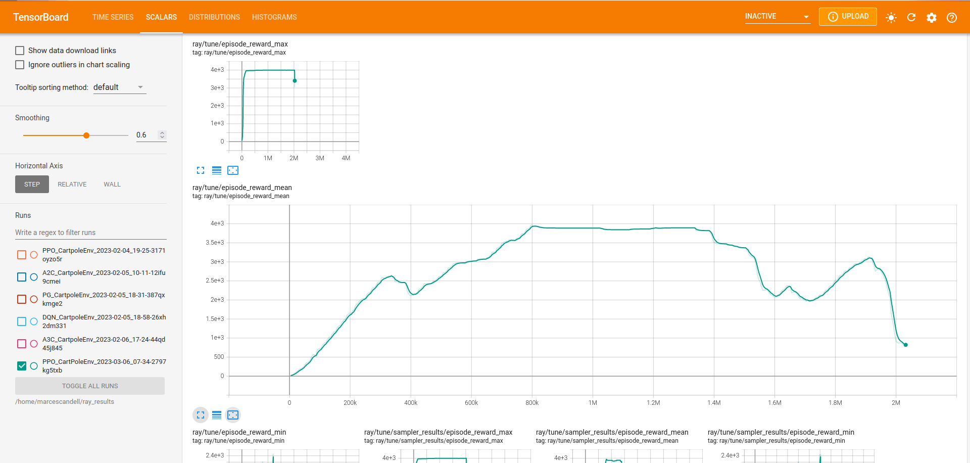
By default, TensorBoard will be saving the training parameters into ~/ray_results. If you want to launch the dashboard and visualise them, you can execute:

tensorboard --logdir=~/ray_results

Tip

Most likely you will be looking to see your policy mean reward as the training progresses. Once your TensorBoard has been launched, you can head to ‘SCALARS’ and apply a filter to display ‘reward’-related parameters (as shown in the screenshot).

The CartPole-v0 implementation

Note

You may find the source code of the CartPole-v0 here.

In this section, you can have a more detailed look on how the CartPole-v0 has been implemented in AnyLogic. Before that, though, you should have connected your AnyLogic model correctly using the ALPypeRLConnector agent. Click here to review how this is done.

Once setup properly, we can continue implementing the required functions by ALPypeRLClientController interface:

Warning

Adding and implementing ALPypeRLClientController is crucial as it will be used by the ALPypeRLConnector to drive the simulation.

void takeAction(ActionSpace action). This function takes ALPypeRLConnector.ActionSpace as an argument.

Note

ActionSpace class has been build around the assumption that actions can be:

A discrete value (or integer) which you can access by calling int getIntAction() as shown in the CartPole-v0 example.

A continuous value, accessible by calling double getDoubleAction(). Check the CartPole-v1 example.

An array of doubles. accessible by calling double[] getActionArray(). Check the CartPole-v2 example.

Warning

The method that you are calling should be consistent with the action_space that you defined in the custom environment that inherited BaseAnyLogicEnv (in your python script).

For example, calling getIntAction only makes sense if you have defined a spaces.Discrete(n). In case there is a missmatch, an exception will be thrown.

Following is the code used for CartPole-v0 example in AnyLogic:

// Take action and process
switch (action.getIntAction()) {

    case 0:
        cartPole.applyForce(-1);
        break;

    case 1:
        cartPole.applyForce(1);
        break;
}

// Check if cartpole has reached max steps
// or has reached position or angle boundaries
boolean exeedPhysLim = cartPole.getXPosition() < -X_THRESHOLD
                    || cartPole.getXPosition() > X_THRESHOLD
                    || cartPole.getAngle() < -THETA_THRESHOLD
                    || cartPole.getAngle() > THETA_THRESHOLD;
boolean exeedTimeLim = time() == getEngine().getStopTime();

// Compute rewards and check if the simulation is terminal
if (!exeedPhysLim && !exeedTimeLim) {
    // Set reward
    reward = 1;
} else {
    // Set reward
    reward = exeedPhysLim ? 0: 1;
    // Finish simulation
    done = true;
}

double[] getObservation(). In CartPole-v0 example, 4 parameters will be collected and returned in array form:
- X position.
- Linear velocity.
- Pole Angle.
- Angular velocity.
The body of the function is pretty straight forward:
return new double[] { cartPole.getXPosition(), cartPole.getLinearVelocity(), cartPole.getAngle(), cartPole.getAngularVelocity() };
double getReward(). As you saw in the code above, a reward of 1 is collected for every step of the simulation where the cart and the pole are within the set boundaries. That is why the reward is a local variable that is set when on takeAction function.
boolean hasFinished(). Just like getReward, there is a local variable done that will indicate if the model has exceeded the set boundaries or it has reach the end of the simulation clock. It is set in takeAction.
Important

You must return true when the simulation has reached the end. Failing to do so will result in your simulation training geting stuck as exposed here.

You can reuse the following code:
// [...] boolean exeedTimeLim = time() == getEngine().getStopTime(); return exeedTimeLim /*[&& other conditions]*/;

How to train your first policy. The CartPole-v0 example.

Create the Action and Observation spaces

Action space

Observation space

Wrap your CustomEnv around the BaseAnyLogicEnv

Inherit BasicAnyLogicEnv

Call create_custom_env

Policy configuration and training execution

Track your training progress using tensorboard

The CartPole-v0 implementation

Wrap your `CustomEnv` around the `BaseAnyLogicEnv`

Inherit `BasicAnyLogicEnv`

Call `create_custom_env`

Track your training progress using `tensorboard`